
Update April 27th: we redid the benchmark after applying infrastructure updates and optimisations, resulting in a ~2x faster total runtime of 1:37 h (previously 3:17 h).
This article will walk you through the analysis of a small dataset of a GPCR sample (GLP-1 receptor bound to GLP-1, EMPIAR-10673). The purpose of the analysis is to find suitable parameters, get an idea of your sample quality and obtain a well resolved initial map. All the data presented here was analyzed on CryoCloud, but the principles apply to other analysis pipelines. The article will also give you an impression of CryoCloud’s performance.
Before we dive in, a short disclaimer: for this article we used the dataset EMPIAR-10673 (Danev et al., 2021) containing a highly optimized and well-behaved sample. That means that you might not get comparably high resolutions with your data, but following these steps, you should be able to quickly characterize your sample in regard to particle density, homogeneity, and its propensity to yield well resolved classes. The aim of this article is to highlight important steps during data analysis, and demonstrate that a readout can be obtained quickly without beating your data to death. This will allow you to either get back to the bench quickly to optimize your sample, or, if more data is needed, already plan your next microscope session.
And now let’s get started.
Divide and conquer: select a subset and don’t optimize analysis on a large dataset
This is one of the well-known, yet often ignored best practices: rather than crunching your whole dataset, you can save a lot of time by choosing a subset that includes an adequate number of particles for initial parameter analysis and screening of your data. I sometimes catch myself or see students ignoring this practice, tempted by the prospect of smoothly progressing through the analysis and quickly obtaining a high-resolution structure. However, the harsh reality is that structure determination is an iterative process, and the majority of datasets will not result in a high-resolution structure right from the start.
For our analysis, we picked a subset of 300 movies from the EMPIAR-10673 dataset, which contains 5,739 movies in total. We selected the first 300 movies from the uploaded dataset (rather than a random subset), to mimic a scenario where one is either waiting for the transfer of the acquired dataset to complete, or analyzing the initial movies that are transferred live from the ongoing microscope session.
We first ran Motion Correction and CTF Refinement, which were both finished in 14 minutes (you can find all runtimes and job parameters at the end of the article), and then excluded micrographs with a maximum resolution lower than 3.5 Å, as done in the publication by Danev et al.. This resulted in 213 movies – a relatively high exclusion rate, but not unusual for the start of a session where acquisition has often not stabilized yet or is interrupted by checks (see Figure S1).
Get your picking right
Next, we continued with Particle Picking. Unlike in the original publication, where Relion’s 3D reference picking was used, we used Relion’s Laplacian-of-Gaussian (LoG) particle picker. The LoG based picker picked 174k particles in under 2 minutes. We tested reference-based picking in parallel and compared the results later. Reference-based picking took considerably longer (29 min vs 2 min) and visual inspection showed similar results.
Both picking approaches resulted in a comparable number of particles/micrographs and keeper rate after two rounds of 3D classification (260 vs. 306 particles/micrograph and 31.6 % vs. 38.3 % keeper rate for LoG & reference-based picking respectively). The resolution in the final reconstruction, however, was lower for the particles picked using a reference compared to the particle set obtained from the LoG picker (4.17 Å vs 3.54 Å; see Figure S2).
Getting a clean particle set and obtaining an initial low-resolution map
Next, we extracted the 174,928 picked particles from the LoG picker at a pixel size of 3.03 Å (70 pixel box size). For initial analysis, a pixel size of 2- 4 Å will not only be more than sufficient, but save you time, increase the signal in your data, and help you interpret the results. After extraction, we ran two subsequent rounds of 3D classification with 3 classes each (45 min total). The first round of Class3D resulted in one well-defined class average resolved at 9.24 Å (72.2 % of particles) showing secondary structure features (Figure 1). This class was selected for a second round of 3D Classification, which resulted in a one well-defined class (9.66 Å, 43.5 %) showing a better resolved transmembrane bundle which was selected for subsequent refinement. At this point, we selected 55,366 particles out of the initial set of 174k particle.
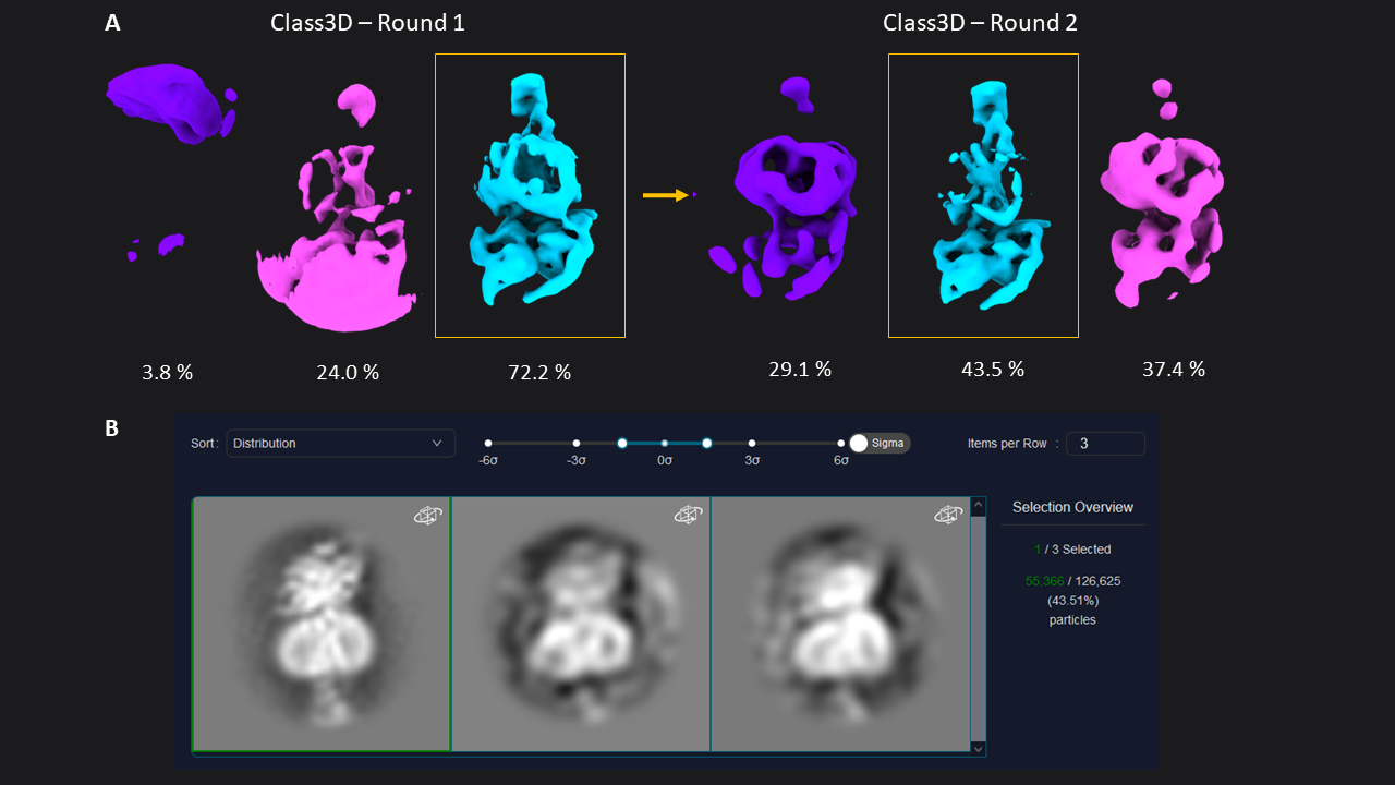 Figure 1: 3D classification of particles and class selection in CryoCloud. A) The set of extracted particles (n= 174,928; box size = 70; pixel size = 3.03 Å) was subjected to two rounds of 3D classification. The well-defined class from the first round was used as input for the second round, resulting in a well-defined class average from a subset of 31% of the total picked particles (selected classes in yellow boxes). B) 3D Class selection panel in CryoCloud - one of several interactive jobs with a custom developed interface, providing sorting of classes and contrast adjustment, and displaying class metadata and total number of picked particles in this case.
Obtaining a high-resolution map
Next, we extracted the 55,366 particles at a smaller pixel size (1.33 Å, 160 pixel box) and subjected this particle set to two rounds of 3D refinement (41 min total). The first round was run with a mask including the membrane micelle. It resulted in an average resolved at 4.34 Å. For the next refinement round, we created a mask excluding the micelle using the map from the last refine 3D job, and also used solvent-flattened FSC’s during 3D refinement. This resulted in a map at 3.54 Å resolution, which we sharpened using Relion’s Post-Processing. The resulting map shows well-defined sidechain densities as expected at this resolution (Figure 2; you can also download the map at the bottom of the article).
We stopped at this point and did not continue with other post-processing jobs (polishing, CTF refinement). If you did select a subset of your full dataset, achieving this resolution is a good point to apply your protocol to the full dataset rather pushing the resolution of the subset. We will cover that part in our next article.
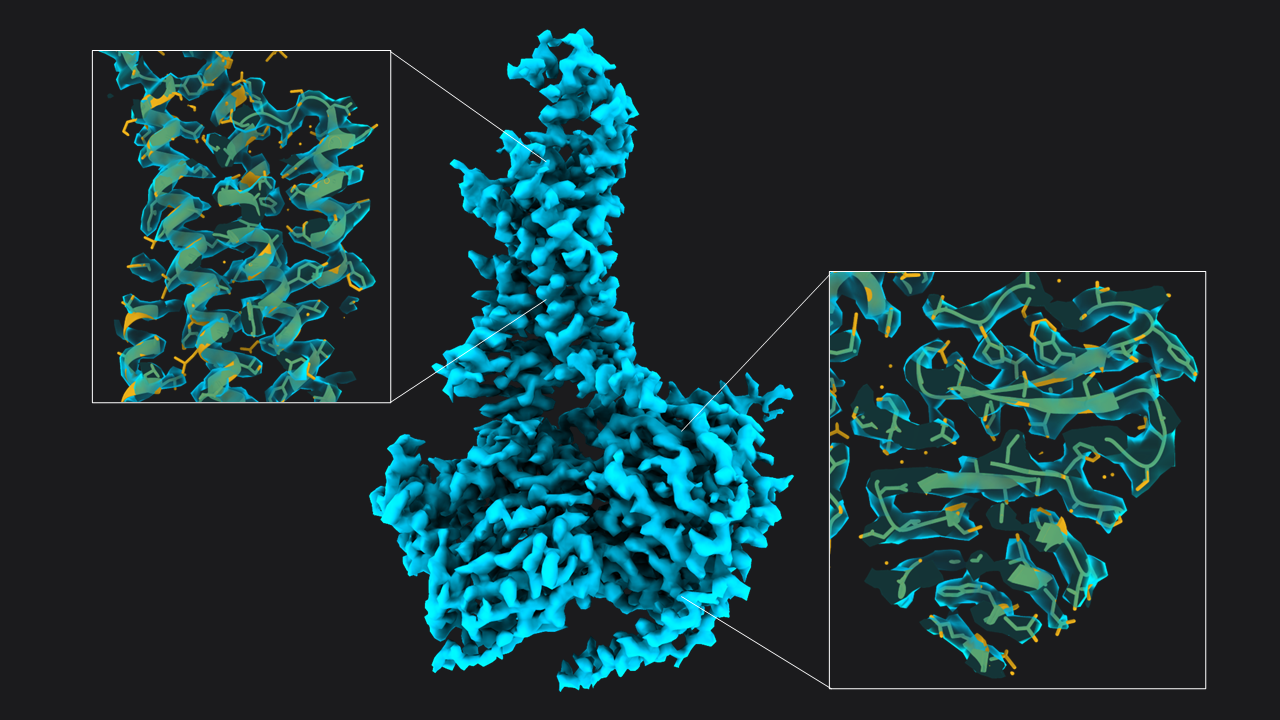 Figure 2: Structure of GLP-1-R bound to GLP-1 at 3.54 Å resolution. Map obtained from ~55,366 particles (pixel size = 1.33 Å, box = 160 pixels) after two rounds of 3D refinement and post-processing. Boxes show slices through the map overlapped with the atomic model (PDB 6x18).
Wrap-up
Excluding short jobs like selection, mask creation and post-processing the whole analysis (9 jobs) was done in a total runtime of 97 minutes on CryoCloud (Figure 3).
Stay tuned for our next article, in which we will run the analysis on the full dataset, and also include post-processing steps (polishing & CTF refinement) to push the resolution even further. If you have any questions, or would like to leverage CryoCloud for your data analysis, get in touch by shooting us a mail at hi@cryocloud.io.
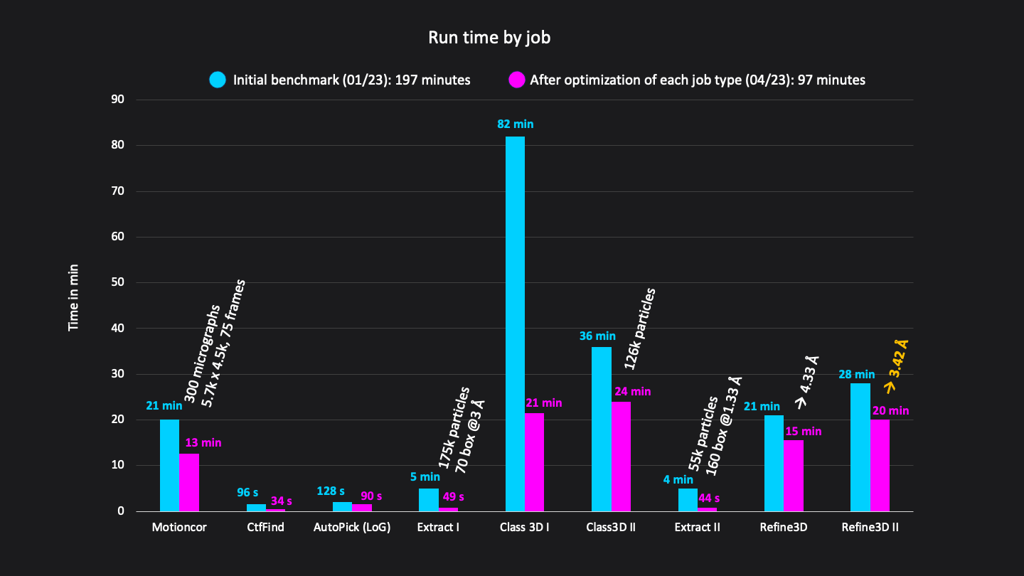 Figure 3: Runtimes of each job in minutes. Excluding short jobs like selection, mask creation and postprocessing the whole analysis workflow consisted of 9 jobs and was done in a total run time of 192 minutes on CryoCloud.